If latency is the problem, I’d fix the bottleneck first: routing for queue jams, stage splits for slow pipelines, caching for repeat work, batching for load spikes, precision cuts for memory limits, and placement for network delay.
This article compares 6 ways to cut latency in multimodal systems that handle text, images, audio, and video. The main takeaway is simple: no single method wins everywhere. Some methods lower TTFT, some protect p95 latency under load, some push more throughput from the same GPUs, and some trade quality for lower cost.
Here’s the short version:
- Modality-aware routing helps when text requests get stuck behind image, audio, or video jobs.
- Stage disaggregation helps when one slow step, like video encoding, stalls the whole flow.
- Caching gives the biggest gains on repeat inputs, prefixes, or retrieval results.
- Batching and admission control help under heavy concurrency, but poor queue rules can hurt TTFT.
- Compression and lower precision cut memory use and compute time, but low-bit formats can trim quality.
- Deployment and hardware placement set the floor for latency because network hops and co-tenancy add delay.
A few numbers stand out:
- Routing cut average TTFT by 14% and P99 TTFT by 32% in one serving study.
- Stage splitting and overlap cut TTFT by up to 4.2× on vision-language workloads.
- Cache-heavy setups showed 3.72–4.86× TTFT gains and up to 80% higher throughput.
- Continuous batching improved p99 latency and TTFT by 2.2–2.3× versus fixed batching.
- FP8 serving showed about 30% lower TTFT and 2.2× throughput on large models.
- Better placement and split modality pools cut TTFT by 27% to 46%, depending on the model.
If I had to reduce this article to one rule, it would be this: move less work, queue work better, and run the work closer to the right hardware.
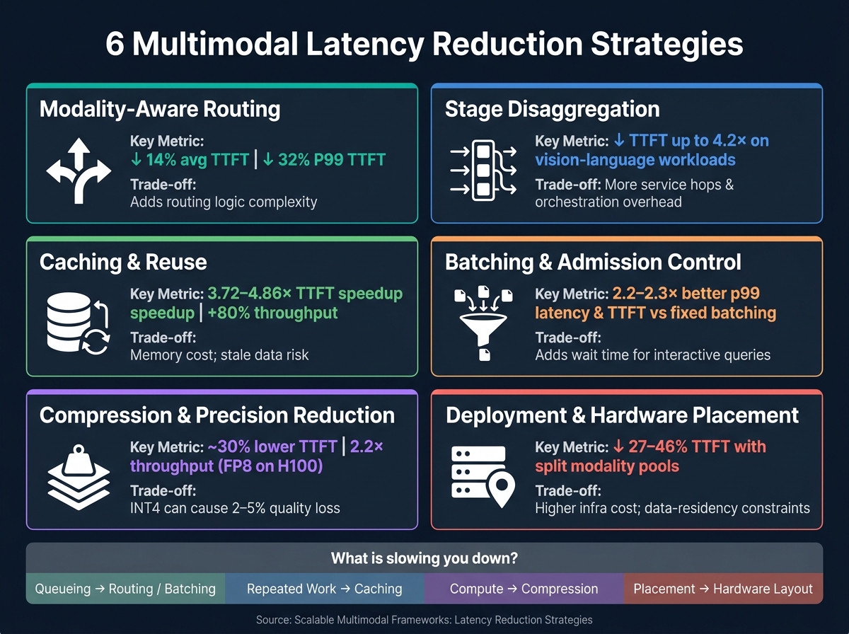
6 Multimodal Latency Strategies: Performance Gains at a Glance
AI Infra at Scale: Inside High-Throughput, Low Latency LLM Performance
sbb-itb-738ac1e
Quick Comparison
| Strategy | Best For | Main Latency Win | Main Trade-Off |
|---|---|---|---|
| Modality-aware routing | Mixed traffic | Less head-of-line blocking | More routing logic |
| Stage disaggregation | Uneven pipelines | Better overlap across stages | More service hops |
| Caching | Repeat traffic | Big TTFT drop on hits | Memory use, stale data |
| Batching + admission control | High concurrency | Better queue control and GPU use | Added wait time |
| Compression + precision reduction | Memory-bound inference | Lower per-request compute time | Possible quality loss |
| Deployment + placement | Distributed systems | Less network and cross-node delay | More infra cost |
So if you’re tuning a multimodal stack, I’d start by asking one question: Is the delay coming from queueing, repeated work, compute, or placement? That answer usually tells you which of the six methods to use first.
1. Modality-Aware Routing and Scheduling
This strategy goes after head-of-line blocking first. Then it helps spread work more evenly across workers built for each modality.
The idea is simple: route each request by modality before it hits the main model. A lightweight classifier looks at the input type and metadata, then sends text, image, audio, and video requests to the right workers. Text goes to LLM workers tuned for fast prefill and decode. Images go to dedicated vision nodes. Audio and video go to ASR systems or feature extractors.
TTFT Impact
When all modalities share the same queue, heavy image or audio jobs can hold up text requests. That’s classic head-of-line blocking. Modality-aware routing breaks that link.
Research on ModServe, a scalable serving system for large multimodal models, found that adding modality-aware scheduling alone cuts average TTFT by 12% and P99 TTFT by 25%. Full modality-aware routing cuts average TTFT by 14% and P99 TTFT by 32%.[12]
p95 Latency Under Load
In isolated vision tests, latency often falls between 280 and 520 ms. In enterprise multimodal pipelines at production load, though, p95 can reach around 4.2 seconds.[7]
Separate modality queues, paired with least-outstanding-requests (LOR) routing inside each modality pool, go straight at that gap. AWS has reported that LOR-based routing can improve end-to-end p99 latency by 4–33% and throughput per instance by 15–16%.[3] So if image traffic suddenly spikes, image-heavy requests can go to whichever image node has the smallest queue instead of piling onto a busy worker.
Routing cuts queue contention. It doesn’t erase the cost of later stages.
Throughput Scaling
Dedicated pools let each modality scale on its own hardware. That means image or audio traffic is less likely to choke text decode when load climbs.
Accuracy/Resource Trade-Off
This setup can also cut cost in a big way. Routing simple classification tasks to a smaller model priced at $0.25 per million input tokens, instead of a larger model at $3.00 per million, gives roughly a 12× cost reduction with little quality loss for those tasks.[8]
The trade-off is straightforward: quality versus latency. If a specialist encoder misses a quality threshold, the system can fall back to the larger multimodal model. There’s another catch too. Routing that keeps inputs in their native format can bring a 1.8× latency increase compared with unified-routing baselines, so careful profiling matters before locking in that setup.[10][11]
Once routing is split out, the next gains come from breaking the pipeline into stages and overlapping the work.
2. Stage Disaggregation and Pipeline Overlap
Routing clears the traffic jam at the front door. Stage disaggregation deals with the slowdowns that happen inside the pipeline.
The idea is simple: split encoding, prefill, and decode into separate services so a slow step doesn’t hold up a fast one. Each stage gets its own queue and its own scaling policy. The system then passes intermediate outputs – like embeddings and token sequences – through RPC calls or queues. This setup helps most when one stage takes much longer than the others.
TTFT Impact
For video-heavy inputs, encoding can take up to 50% of TTFT. That means one slow branch can drag the whole request behind it. By isolating encoding, token generation can begin earlier while slower modality branches keep running in parallel.[15][18]
ElasticMM, a multimodal LLM serving system, pairs modality-aware decoupling with stage-level elastic scheduling. On the ShareGPT-4o dataset, it cut TTFT by up to 4.2× for Qwen2.5-VL and 3.5× for LLaMA3.2-Vision compared with vLLM. On VisualWebInstruct, the same system delivered 3.7× and 2.9× gains for those models.[13][16] The main win comes from removing synchronization points.
p95 Latency Under Load
This split also helps with tail latency when traffic comes in bursts. Stage-local queues keep one spike from rippling through the whole system. In pipeline-parallel setups, p95 stays much closer to median latency. Monolithic systems, by contrast, tend to spike far higher under load.[14]
Throughput Scaling
Disaggregation also lets you overlap work that would otherwise run one step at a time. While one request is decoding, the next can be in prefill, and another can still be encoding.
Studies of pipeline-parallel LLM inference report 1.5–3× throughput gains over sequential execution at similar latency targets.[14] And in ensemble pipelines, GPU-only execution can cut end-to-end latency by 6× compared with mixed CPU/GPU execution.[17]
Accuracy/Resource Trade-Off
A practical way to manage cost is to use low precision for broad filtering, then keep full precision for borderline or high-value requests. It also helps to cap in-flight requests and pass compact intermediates, such as token IDs, so memory pressure doesn’t become the next choke point.
Once stages are split, the next latency gain comes from reusing work across requests.
3. Caching and Reuse Across Modalities
Caching cuts repeated work. If the same input, prompt prefix, or retrieved item shows up again, you can reuse encoder outputs, KV states, and retrieval embeddings instead of doing the whole job from scratch. In multimodal systems, that makes caching one of the biggest levers for latency.
TTFT Impact
The biggest gains show up when the repeated unit stays the same: an image, a prompt prefix, or a retrieved embedding. Systems like VLCache do this by hashing and caching encoder outputs. On repeated image inputs, it computes only 2% of vision tokens and reuses 98%, which can skip the vision encoder pass on cache hits.[23]
LMCache uses a similar approach for multimodal vLLM workloads. In practice, repeated image requests drop from tens of seconds to about 1 second when users view the same image again.[21][22][24] For long shared prompts, CacheTune reports 3.72–4.86× TTFT speedup and 3.93–6.21× throughput increase, with generation quality staying close to full recomputation.[25]
p95 Latency Under Load
Cache hits don’t just help the average. They also smooth out the tail.
A warm cache lets a request avoid the slow path: re-running a vision encoder, recomputing a long prompt prefix, or hitting a vector database again. Without caching, real enterprise deployments at typical U.S. concurrency levels see p95 latencies of about 2.5–4.5 seconds for multimodal workloads.[7] Push vector and prefix caching hard enough, and cold-path latency can fall by 35–45%, while p95 drops by 25–35%.[7]
Throughput Scaling
Caching also frees GPU time that would have been spent on repeated encoding. LMCache reports about 80% higher throughput along with its 6.7× TTFT improvement.[2]
For RAG-heavy pipelines, the pattern is similar. RAGCache reaches up to 2.1× throughput by caching intermediate KV states and retrieval results. Proximity cuts database calls by 77–79% and retrieval latency by 59–72.5%, with less than a 1% accuracy drop.[26][27] Another practical move is to precompute embeddings for high-traffic assets. That turns repeat queries into simple lookups and helps push more traffic through fixed GPU capacity.[7][19]
Accuracy/Resource Trade-Off
For deterministic stages, cached outputs usually stay very close to fresh runs, with no meaningful accuracy loss.[20] The bigger risk is stale context. If you reuse a cached embedding after the source content changes, the model is working from old information.
There’s also a memory cost. Fine-grained caches, like per-image or per-video-segment caches, can improve hit rates, but they can drive memory use up to 100× higher than text-only workloads because multimodal KV caches are much larger.[15]
A few rules help here:
- Use LRU eviction to clear low-value entries.
- Set modality-aware TTLs.
- Keep static assets cached longer.
- Keep text TTLs short.
When cache hit rates stop improving the tail, batching and admission control become the next lever.
4. Batching and Admission Control
Once caching is in place, queue pressure becomes one of the biggest drivers of latency. That’s where batching and admission control come in. They solve two different problems. Batching decides how requests are grouped and run. Admission control decides which requests are allowed into the system in the first place.
TTFT Impact
Batching can help or hurt time to first token (TTFT).
On one hand, it improves GPU use by spreading overhead across many requests. On the other, it can make each request sit in line longer before work even starts. A 7B benchmark shows the upside clearly: per-request latency drops from 976 ms at batch size 1 to 126 ms at batch size 8 because compute overhead gets amortized.[9]
That said, multimodal workloads often feel the downside more than text-only systems. Why? Preprocessing time can vary a lot by input type. If one request has a large image or longer audio clip, a fixed batch may end up waiting for that slowest item before execution begins.
A better approach is continuous (in-flight) batching. Instead of waiting for a full batch to finish, new requests can join a running batch at decode-step boundaries. Paired with paged attention, this method delivers 2.2–2.3× better p99 latency and TTFT than fixed batching.[6] For interactive use cases, that kind of gain matters. The MLCommons MLPerf 5.1 interactive benchmark treats TTFT ≤ 500 ms at p95 concurrency as a key target.[2]
p95 Latency Under Load
The same queue effect shows up in the tail. One detailed LLM latency breakdown makes the problem plain: median queue wait is about 20–25 ms, but p95 queue wait climbs to 310 ms, while prefill and decode times stay fairly steady.[28] In other words, if p95 is bad, the model may not be the main issue. The queue policy probably is.
Admission control helps by putting limits on:
- concurrent requests
- batch token budgets
- priority rules
That keeps interactive traffic from getting stuck behind long-running jobs.
For multimodal systems, complexity-aware admission control is especially useful. The idea is simple: estimate compute cost before accepting a request, based on things like image resolution, audio length, or visual token count. That gives the system a better shot at keeping p95 under control. InternVL3 multimodal inference with token-budget-aware batching cut p95 latency by about 50% and cut energy use by about 50% compared with mixed batching across batch sizes 4–64.[29]
Throughput Scaling
Larger batches usually improve occupancy and reduce overhead, but the gains level off fast. In multimodal systems, batches get fragmented more easily than in text-only workloads, so that limit tends to show up earlier.
In practice, micro-batching – often groups of 2–8 requests – is a solid middle ground on memory-limited hardware. It gives better utilization without pushing TTFT too far. For offline work, such as bulk video tagging or large document analysis, larger static batches tuned to the accelerator’s memory limits make more sense. Those jobs can accept longer waits per request if total throughput is higher.[9][30][31]
Accuracy/Resource Trade-Off
Higher throughput often comes from tighter system limits, and that’s where quality can start to slip.
Batching by itself does not lower model accuracy. The issue is the set of choices teams make to keep latency in check. A system may reduce input resolution, trim context, or skip lower-priority modalities. Those moves save time and compute, but they can also weaken output quality, especially for tasks that rely on fine visual or audio detail.[1][9]
A practical setup is to split traffic into separate service tiers:
- high-fidelity for quality-sensitive jobs
- low-latency for interactive traffic
Admission control can then route each request to the right model variant based on SLA and cost limits.[1][9][32]
5. Compression and Precision Reduction
Once queue pressure is in check, compression helps cut the amount of work each request has to do. Lowering weight precision and compressing inputs reduces memory use, speeds up compute, and trims latency – but there’s always a quality trade-off to watch. At this point, it’s the last big per-request lever after routing, overlap, caching, and batching are already dialed in.
TTFT Impact
Lower-precision weights make the model smaller in memory and speed up matrix math on Tensor Core hardware. In practice, moving from FP32 to FP16 or BF16 often leads to about 20–40% lower TTFT for large models when memory bandwidth is the main limit.
INT8 quantization can push this further. With tuned kernels such as TensorRT-LLM, TTFT can drop by another 20–30%. And if you quantize vision or audio encoders to INT8, encoder-side latency can fall by 30–50% for image or audio prompts[34].
A good example comes from Databricks’ FP8 serving report for Llama 2–70B on NVIDIA H100. FP8 delivered roughly 30% lower TTFT, a 2.2× throughput gain, and about 50% model size reduction compared with FP16[35].
p95 Latency Under Load
Precision reduction helps tail latency the most when memory bandwidth – not raw compute – is the bottleneck. With FP16 or BF16, production systems often see 20–35% lower p95 latency at similar traffic levels versus FP32. Why? Because more work fits on each GPU, and there’s less spillover into slower execution paths[34].
NVIDIA’s NVFP4 KV-cache format goes a step further. It reportedly delivers 20% higher cache hit rates and 3× lower latency at large batch sizes compared with FP8 KV-cache[2]. That’s an important point: compressing the cache, not just the weights, can cut tail latency too.
For inputs, use formats like WebP or JPEG for images and Opus for audio. Just keep decompression off the critical path. Otherwise, you save time in one place and give it right back in another.
Throughput Scaling
Lower-bit formats let each GPU handle more tokens per second before memory becomes the limiter. FP16 and BF16 often deliver around 1.5–2× more tokens/sec per GPU for large LLMs. INT8 can add another 30–50% throughput in tuned frameworks[34].
A common production setup is mixed precision:
- Vision and audio encoders run at INT8
- The main language model stays at BF16 for stability
That split tends to give a good balance between speed and output quality.
Accuracy/Resource Trade-Off
FP16 and BF16 usually keep quality intact. INT8 tends to stay under 1% loss. INT4 is where the risk starts to climb, especially for reasoning-heavy work and fine-detail vision tasks[34].
If a workload can tolerate a 7% accuracy drop, latency cuts of up to 60% may be possible[33]. That can be worth it in lower-stakes cases. In safety-critical settings, though, the safer default is BF16/FP16, with selective INT8 only for parts that matter less. For less sensitive workloads, INT4 or FP8 can work – as long as you watch the numbers and fall back to higher precision if TTFT, p95, or quality metrics drift past set thresholds.
| Precision Level | Typical Quality Loss | Typical Throughput Gain | Best Fit |
|---|---|---|---|
| FP16 / BF16 | Minimal | 1.5–2× | Default |
| INT8 | Usually under 1% | 30–50% higher in optimized frameworks | High-concurrency interactive |
| INT4 / FP4 | 2–5% | Highest potential | Only when loss is acceptable |
Even with heavy compression, placement still sets the latency floor.
6. Deployment Pattern and Hardware Placement
Even after you compress weights and tune batch sizes, deployment layout still sets the latency floor. At this point, where hardware sits and how requests move through the system become the last big knobs for cutting queueing, RPC, and network delay.
TTFT Impact
Putting pipeline stages on the same machine is one of the biggest levers for TTFT. If pre-processing, model inference, and post-processing all run on the same physical node, you remove inter-node RPC overhead and the wait time between stages. That can save about 5–30 ms per request compared with cross-node setups.[39]
Cross-node placement also brings network jitter into the picture. Under load, that extra variability can push TTFT up fast.
Location matters too. Users on the West Coast may see about 30–80 ms of extra round-trip latency compared with a centralized us-east-1 cluster.[39] That said, cold starts on the selected hardware are often the bigger TTFT driver.[39]
Splitting image and text pools at deployment led to large TTFT gains. For Llama 3.2, it reduced average TTFT by 27% and P99 TTFT by 42%. For InternVL, the drops were 46% and 47% versus vLLM.[4][5]
p95 Latency Under Load
This is where deployment choices stop looking abstract and start hitting users. Tail latency tends to expose every weak spot in the stack.
One of the fastest ways to drive up p95 is to share GPUs with batch jobs. Co-tenancy can increase p95 latency by 2–5× under load.[39] For production traffic that matters, dedicated GPU nodes separated from offline jobs are usually the safer call.
A tiered GPU pool can help a lot:
- One pool for lighter text-only models
- Another for heavier vision or audio models
- Independent autoscaling for each pool
That setup can cut p95 latency by 25–40% for mixed workloads because large image batches no longer hold up short text requests.[39]
ElasticMM pushes this idea further with elastic resource allocation across modality-specific components. It reports up to 4.2× TTFT reduction and 3.2–4.5× higher throughput than vLLM while still meeting latency SLOs.[40]
The next issue is simple: what hardware tier can take that load without hurting accuracy?
Throughput Scaling
In vLLM-style systems, a common rule is to match tensor parallelism to the number of GPUs per node and pipeline parallelism to the number of nodes. That keeps inter-node communication overhead in check while still letting you scale out for larger models.[36][37][38]
For audio workloads, a hybrid edge-plus-cloud setup often works well. Run audio feature extraction locally, then send the higher-level semantic work to centralized GPUs. This avoids 20–40 ms of streaming delay compared with uploading raw audio first.[39] For the same GPU budget, that split can deliver 1.5–3× higher throughput.[39]
Accuracy/Resource Trade-Off
Your hardware tier shapes how much latency you can shave off before accuracy starts to slip. If the workload involves enforcement or compliance, central H100/A100 clusters usually make more sense. Edge deployments can be faster, but that speed often comes with some accuracy loss.
| Hardware Tier | Typical Use Case | Precision | Accuracy Risk |
|---|---|---|---|
| H100 / A100 (central cluster) | Enforcement, compliance, high-stakes multimodal | FP16 / BF16 | Minimal |
| L4 / T4 (mid-range GPU) | Interactive text + light vision | INT8 / mixed precision | Low |
| Edge CPU / small accelerator | Real-time UX, mobile | INT4 / INT8 | Moderate |
Many U.S. organizations use tiered service levels. One pipeline is slower but more accurate for audits and enforcement. Another is faster, with moderate accuracy, for real-time user experiences.
Criterion-by-Criterion Comparison
The tables below compare the six strategies across TTFT, p95 latency, throughput, and accuracy/resource trade-offs. Think of them as a trade-off map. The best latency lever changes based on the bottleneck: queueing, compute, or placement.
TTFT Impact
When image encoding takes the most time, strategies aimed at the encoder tend to have the biggest effect on TTFT.
| Strategy | TTFT Impact | Key Driver |
|---|---|---|
| Modality-Aware Routing & Scheduling | Modest – the main upside comes from queue isolation | Removes head-of-line blocking, so text requests no longer sit behind image jobs |
| Stage Disaggregation & Pipeline Overlap | Moderate TTFT gain on hot paths | Separate stage queues and overlap encoding with decoding |
| Caching & Reuse Across Modalities | Largest TTFT gain on hits; cold misses stay near baseline | Retrieval replaces computation on cache hits |
| Batching & Admission Control | Weak TTFT unless continuous batching is used | Requests wait until a batch forms, so latency is traded for steadier throughput |
| Compression & Precision Reduction | Moderate – most helpful when first-token generation is compute-bound | Faster compute on quantized weights; less help when networking or cold start is the bottleneck |
| Deployment Pattern & Hardware Placement | Varies by placement – edge-first cuts network delay; cloud-first adds RTT and cold-start overhead | Physical distance to the user and cold-start behavior shape TTFT |
p95 Latency Under Load
TTFT only shows one part of the picture. Tail latency tells you if the system can stay responsive when concurrency stays high. The scenario below assumes a mixed U.S. production workload: about 50% text-only prompts, 30% image requests, and 20% video captioning, all under sustained high concurrency.
| Strategy | p95 Behavior Under Load | Notes |
|---|---|---|
| Modality-Aware Routing & Scheduling | Stable – lighter text traffic stays responsive even as heavier modalities grow | Heavy workloads do not starve lighter ones |
| Stage Disaggregation & Pipeline Overlap | Improves when hot stages scale independently; can get worse if orchestration overhead is not tuned | Cross-service hops add jitter when services are not colocated |
| Caching & Reuse Across Modalities | Best latency gains on repeat traffic; weak on cold misses | In-memory, colocated caches matter a lot for the hit path |
| Batching & Admission Control | Strong throughput, weaker TTFT unless continuous batching is used; continuous batching can deliver about 2.2–2.3× better p99 latency and TTFT[6] | Smooths p95 at higher load by cutting queue churn |
| Compression & Precision Reduction | Often lowers p95 for compute-heavy image and video workloads under load[41] | Works best when hardware is set up to use lower precision well |
| Deployment Pattern & Hardware Placement | Varies by placement – edge-first cuts network delay; cloud-first adds RTT and cold-start overhead | Local hardware limits and network swings shape the tail |
Throughput Scaling
After latency, throughput shows which strategy scales cleanly without just moving the bottleneck somewhere else.
| Strategy | Throughput Scaling Shape | Typical Gain |
|---|---|---|
| Modality-Aware Routing & Scheduling | Near-linear per modality when each has dedicated workers and autoscaling | Each modality scales on its own track |
| Stage Disaggregation & Pipeline Overlap | Higher total throughput by scaling bottleneck stages on their own and overlapping work | 30–50% TPS increase reported in microservice-based ML stacks |
| Caching & Reuse Across Modalities | Higher effective throughput per GPU when hit rates are strong | 2–5× throughput improvement on workloads with high cache hit rates[43] |
| Batching & Admission Control | Starts super-linear, then turns sub-linear once the GPU saturates | Batch size 64 can deliver 14× throughput on a single A100, with the expected latency trade-off[42][45] |
| Compression & Precision Reduction | More concurrent streams per GPU; scales well with dynamic batching | Quantized models often show 1.5–3× throughput gains[41] |
| Deployment Pattern & Hardware Placement | Hybrid supports tiered scaling – edge absorbs routine tasks, cloud handles complex jobs | Reduces pressure on central clusters; cloud-first scales by adding instances until budget or capacity becomes the limit |
Accuracy/Resource Trade-Off
This is where engineering judgment matters most. Not every optimization keeps quality the same, and the right choice depends a lot on whether the workload sits in regulated industries or consumer-facing tasks.
| Strategy | Accuracy Impact | Resource Efficiency |
|---|---|---|
| Modality-Aware Routing & Scheduling | Minimal – better routing can make room for heavier models on key modalities | High – fewer GPU cycles are wasted on mismatched workloads |
| Stage Disaggregation & Pipeline Overlap | Minimal – supports specialized high-accuracy submodels per stage | Moderate – more orchestration overhead, but better fault isolation |
| Caching & Reuse Across Modalities | No change for hits; staleness risk in time-sensitive domains like finance, healthcare, and legal | Very high – one GPU serves far more users when hit rates are strong |
| Batching & Admission Control | Model accuracy stays the same; user experience falls when queueing breaks latency targets | High – larger batches improve hardware utilization a lot |
| Compression & Precision Reduction | FP8/W8A8 is near-lossless; INT8 usually costs 1–3% accuracy; INT4 gives the biggest speedup with the highest quality risk – in resource-constrained settings, well-tuned 8-bit and 4-bit models can beat FP16 by avoiding VRAM bottlenecks[44][41] | Very high – about half the memory footprint, with INT8 often delivering about 1.5–2× speedup |
| Deployment Pattern & Hardware Placement | Edge-first often uses smaller or distilled models, trading accuracy for speed; cloud-first serves larger, more accurate models | Hybrid routes high-stakes queries to full-size cloud models and routine tasks to lighter edge models |
Pros and Cons
This section shows where each strategy helps, where it struggles, and when it makes the most sense.
Use the table below to match each option to the bottleneck it addresses: queueing, reuse, compute, or placement. It turns the earlier metric-by-metric review into a simpler decision view.
| Strategy | Primary Gain | Main Limitation | Best Deployment Scenario | Main Risk |
|---|---|---|---|---|
| Modality-Aware Routing & Scheduling | Cuts tail latency by separating light text traffic from heavier multimodal jobs. | Needs dependable modality detection; unclear or mixed inputs can go down the wrong path. | Real-time assistants and multimodal search with very different request types. | Low quality risk; system complexity grows if you add too many specialized routes. |
| Stage Disaggregation & Pipeline Overlap | Cuts tail latency by splitting slow stages and overlapping work. | Orchestration overhead and cross-service hops add jitter; debugging across micro-stages is harder. | High-volume content moderation and recommendation systems with steady workload streams. | Minimal accuracy impact; moderate complexity risk from backpressure failures and uneven stage use. |
| Caching & Reuse Across Modalities | Removes recomputation on repeat assets. | Stale cache risk in time-sensitive domains; distributed cache coherence is costly to maintain. | Media platforms and knowledge bases with repeat access to the same images, videos, or prompts. | No quality change on hits; staleness risk in finance, healthcare, and legal contexts. |
| Batching & Admission Control | Improves throughput by grouping compatible requests. | Adds wait time for interactive queries; aggressive admission control can delay or drop lower-priority traffic. | Back-office and semi-real-time workloads like bulk content classification or email triage. | Little to no direct effect on model accuracy; user experience gets worse when queueing breaks latency SLOs. |
| Compression & Precision Reduction | Lowers inference time by cutting precision and memory pressure. | Heavy quantization can hurt quality in niche modalities and may need retraining or fine-tuning. | Edge deployments, mobile multimodal apps, and cost-sensitive SaaS inference APIs. | FP16/BF16 and conservative INT8 are lower risk; heavier compression can be a bad fit for medical or safety-critical workloads. |
| Deployment Pattern & Hardware Placement | Cuts network and cross-node overhead by placing work closer to the user or on the same node. | Multi-region and edge deployments add cost and data-residency constraints. | Globally distributed, latency-sensitive U.S. products like live video analysis or streaming recommendations. | Specialized hardware and multi-region designs add operational complexity; tensor parallelism usually wins on latency when fast interconnects are available. |
A simple way to read this table: some tactics help you move less work, some help you queue work better, and others help you run the work faster. That distinction matters. If the main issue is repeated inputs, caching helps. If the problem is interactive traffic getting stuck behind heavy jobs, routing or admission control usually does more.
There’s also a tradeoff pattern here that shows up again and again. The strategies that trim latency at the system level, like routing, stage splitting, and hardware placement, tend to add operating overhead. The strategies that cut compute cost, like compression, can chip away at output quality if pushed too far. And the options that improve throughput, like batching, can frustrate users when response-time targets start slipping.
So the best choice usually comes down to one thing: what is slowing you down right now. If the bottleneck is compute, look at precision and placement. If it’s queueing, look at scheduling and batching. If it’s wasted repeat work, caching tends to be the obvious first move.
Conclusion
Pick tactics based on the bottleneck: queueing, reuse, compute, or placement. The right mix depends on where latency is coming from.
For real-time assistants, balance quality and latency by combining modality-aware routing, stage disaggregation, and light admission control. That mix goes straight at head-of-line blocking and pipeline imbalance, which helps keep tail latency low without wasting GPU capacity. Research on this setup shows p99 tail latency drops along with about 3× throughput gains[46].
When interactivity matters less, move the focus from queue control to throughput. For batch workloads, use larger batches, caching, and compression to get the most out of the system when interactive latency is not the main goal. Caching cuts repeated compute. Compression lowers per-request cost when queues start to build.
Mixed enterprise workloads usually call for selective routing, moderate batching, and precision reduction on non-critical paths. The deployment principle is tiered routing across hardware classes, not a fixed workload template.
Use the smallest set of tactics that fully fixes the bottleneck. Stop when the next tactic adds complexity but barely improves latency. At that point, it makes more sense to change the model, hardware, or workload design instead. Route better, overlap stages, reuse work, batch with care, compress where it makes sense, and place hardware well.
FAQs
How do I find the real latency bottleneck first?
Start by separating fast candidate retrieval from precise verification. Use ANN search with HNSW graphs or IVF-PQ indexing to cut down the search space fast, then add a second rescoring stage to verify the best matches.
For better performance, split each pipeline stage into its own container, cache intermediate embeddings with normalized content hashes, and use task-specific AI models instead of oversized general-purpose ones.
Which strategy should I try before changing models or hardware?
Start with a layered architecture. Use ANN search, such as HNSW, to pull likely matches fast. Then run a more exact verification step on that smaller set.
To cut latency and storage use, compress dense embeddings with PQ. You can also apply metadata filters to shrink the search space before retrieval even begins.
If proof of ownership is part of the job, add InCyan’s Idem for multimodal matching and ScoreDetect for tamper-evident blockchain timestamps. That setup keeps the system fast while also supporting copyright protection.
How much quality risk comes with lower precision and compression?
Lower precision and heavy compression can add quality risk. The goal is balance: cut latency without giving up accuracy.
A smart setup is to use fast ANN search for the first pass, then follow it with a lightweight, modality-specific verification step. That gives you speed up front, with a quick check before results move on.
At enterprise scale, performance usually depends on a few practical moves:
- Sharding indices so search load is split across systems
- Batching ingestion to handle high data volume more efficiently
- Caching embeddings with version-aware keys so reused vectors stay aligned with the right model or data version
This kind of setup helps keep retrieval fast and stable as usage grows.